HDB resale prices and hawker centre proximity
Arrow keys or a swipe move between slides. Q, or a tap on the page number, opens the question index and returns from it. Click or tap a figure or a query to enlarge it. Every slide names the report section it comes from.
One decision runs through all four tasks: store every block-to-centre distance and derive proximity from it.
Modelling
Distance is a many-to-many relationship between HDB Block and Hawker Center with one attribute,
distance_m. The class near, medium or far is derived in a view and never stored.
See the ER diagram and the proximity bands.
Population
The pipeline computes the Haversine distance for every geocoded block and centre pair, including pairs beyond 1,000 m.
See the pipeline and coordinate matching.
Queries
Q4 and Q5 pick each block's nearest centre from those rows. They are the slowest queries, and they stay flat while sales grow fourfold.
See Q4 and runtime against size.
Indexing
A composite index in the order of the nearest-centre sort roughly halves Q4 and Q5. A second distance index speeds up Q6.
See the plan change and the recommendation.
Pairs beyond 1,000 m are kept on purpose: a block that is genuinely far from every centre can then be told apart from a block with missing coordinates, which gets an unknown class (NULL) and is never counted as far.
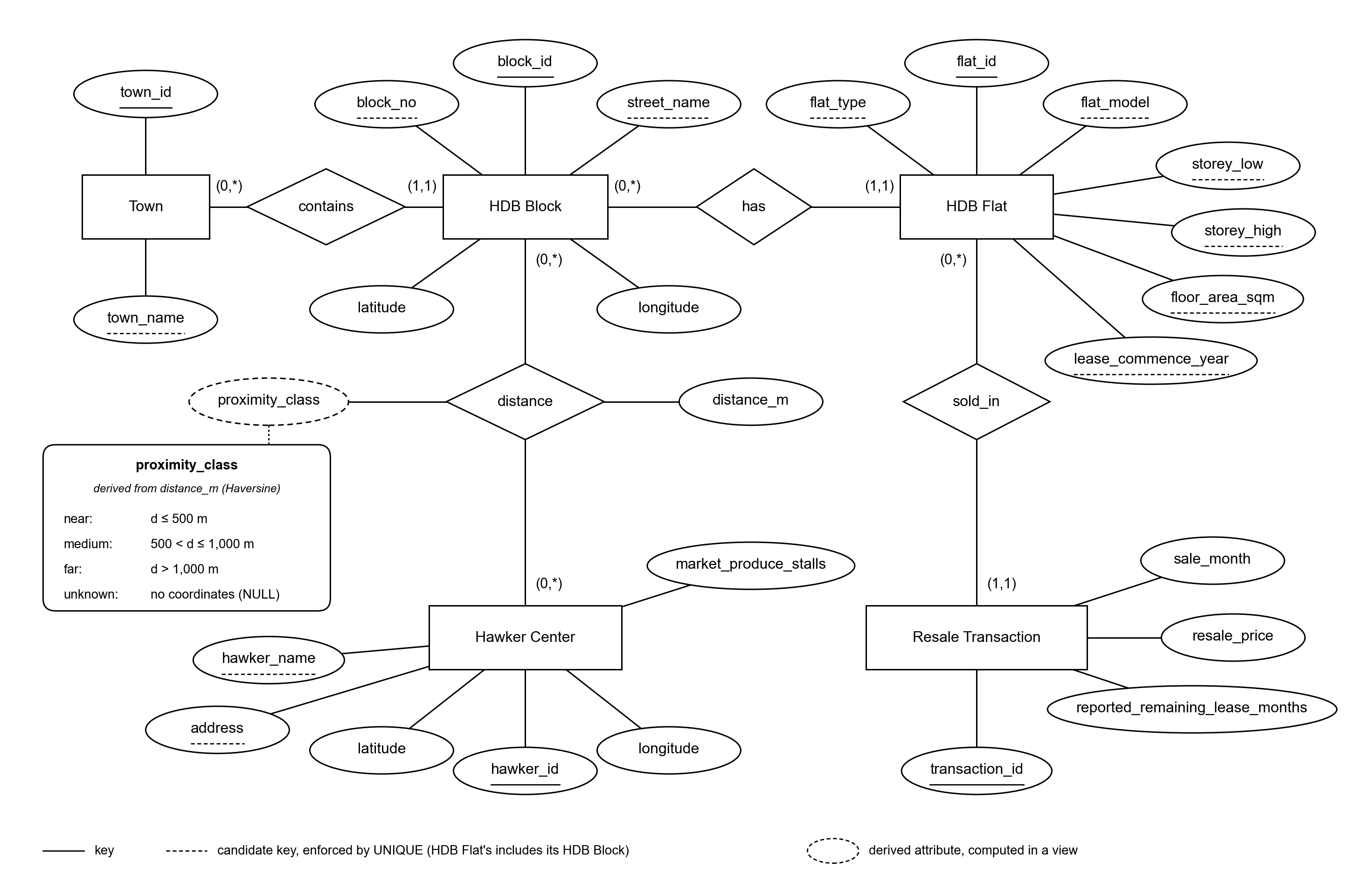
The ER model has five entity types, and proximity is a many-to-many relationship that carries distance_m.
| Relationship | Participation (min,max) |
|---|---|
| Town contains HDB Block | Town (0,*), Block (1,1) |
| HDB Block has HDB Flat | Block (0,*), Flat (1,1) |
| HDB Flat sold_in Resale Transaction | Flat (0,*), Transaction (1,1) |
| HDB Block distance Hawker Center | Block (0,*), Centre (0,*) |
HDB Block is our addition to the four required entities. Coordinates belong to a block, not to a flat, so distance is measured from block to centre.
Zero minimums on distance: a block or centre without coordinates has no distance pair.
Underlines: solid marks the surrogate primary key, dashed the natural candidate key enforced with UNIQUE. Resale Transaction has no natural key in the published data.
Near, medium and far are straight-line distance bands from a block to its nearest listed centre.
Distance: great-circle distance by the Haversine formula with Earth radius 6,371,000 m, computed from stored coordinates and classified before any rounding.
Boundaries: exactly 500 m is near, exactly 1,000 m is medium.
One class per sale: the nearest centre decides. A tie goes to the smaller
hawker_id.
Q5: centres are filtered to market_produce_stalls > 0 first, then
the nearest is chosen. A flat can be near a centre overall yet far from a fresh market.
Unknown: missing coordinates give NULL, never far.
Status: the thresholds are project definitions, not official walking standards.
Each entity type becomes one table, and the many-to-many relationship becomes a table keyed by both foreign keys.
town
hdb_block
hdb_flat
resale_transaction
hawker_center
block_hawker_distance
| View (derived, not stored) | One row per | Used by |
|---|---|---|
| v_block_hawker_proximity | geocoded block and centre pair, with its class | the two views below |
| v_nearest_hawker | block: its nearest centre | Q4 |
| v_nearest_fresh_market | block: its nearest centre with produce stalls | Q5 |
| v_resale_analysis | sale, with town, type, price per m², lease and both classes | Q1 to Q5 |
We checked the functional dependencies against the loaded data before fixing where each attribute lives.
| Question | What all 989,263 sales showed | Consequence in the schema |
|---|---|---|
| Does a block address determine its town? | Yes, for all 10,024 blocks. | town_id belongs in hdb_block, with (block_no, street_name) as a candidate key. |
| Does a block determine the lease start year? | No. Three blocks have two lease years each (114 Jurong East St 13; 21 and 37 Teban Gardens Rd). | lease_commence_year stays in hdb_flat. |
| Do block and sale month determine the remaining lease? | No. 13,668 of 234,380 block-months with a reported lease (5.83%) hold more than one value. | The reported lease stays on each transaction. |
| Can the sale attributes form a key for a transaction? | No. 1,929 sales repeat another row's published values exactly within the same file. | The key is (source_file, source_row): the file name with a hash prefix, and the row number. |
| Is an HDB Flat a physical unit? | It cannot be. No file carries a unit number, only block, type, model, storey range, area and lease year. | hdb_flat is an observable profile with a seven-column candidate key. 147,052 profiles carry the 989,263 sales. |
The dependencies in the report are the declared business
rules. These counts show that the loaded data does not contradict them, and they are why
flat_id does not claim that two sales concern the same dwelling.
Every nontrivial determinant is a candidate key, so all six tables are in BCNF.
| Relation | Determinants of all other attributes |
|---|---|
| Town | town_id; town_name |
| HDB Block | block_id; (block_no, street_name) |
| HDB Flat | flat_id; the seven-column profile |
| Resale Transaction | transaction_id; (source_file, source_row) |
| Hawker Center | hawker_id; (hawker_name, address) |
| Block Hawker Distance | (block_id, hawker_id) |
BCNF asks that the left side of every nontrivial functional dependency is a superkey. Each determinant listed is a key the schema enforces, and no other determinant is asserted: a centre name alone, or a block number alone, identifies nothing.
| What we did not store | Dependency it would add |
|---|---|
town_name inside hdb_block | town_id → town_name, where town_id is not a key of the block table |
| Block coordinates inside hdb_flat | block_id → latitude, longitude, where block_id is not a key |
| Profile attributes inside every transaction | flat_id → profile attributes, where flat_id is not a key |
proximity_class beside distance_m | distance_m → proximity_class, where a distance is not a key |
So the class, fresh-market eligibility and price per square metre are derived in views. The claim covers the six base tables, not the deliberately wide analysis view.
Joins lose nothing: each foreign key is NOT NULL and references a unique key, so the chain Town, Block, Flat, Transaction returns exactly one row per sale.
Constraints reject impossible values, yet all 989,263 source sales load.
| Constraint | In the schema | What it keeps out |
|---|---|---|
| Primary key | bigint GENERATED BY DEFAULT AS IDENTITY PRIMARY KEY, with CHECK (id > 0) |
Rows without a stable identity. |
| Candidate key | UNIQUE (block_no, street_name), UNIQUE (source_file, source_row), and one per table |
The same block, profile, centre or source row loaded twice. |
| Foreign key | town_id bigint NOT NULL REFERENCES hdb_hawker.town(town_id), default NO ACTION |
Orphan rows, and deleting a town, block, profile or centre still in use. |
| Domain | flat_type IN ('1 ROOM', … 'MULTI GENERATION')floor_area_sqm BETWEEN 20 AND 400resale_price BETWEEN 1000 AND 5000000sale_month >= DATE '1990-01-01' and day = 1 |
The label 'four room', an area of 999,999 m², a sale month in 1850. |
| Location | latitude BETWEEN 1.1 AND 1.5, longitude BETWEEN 103.5 AND 104.1(latitude IS NULL) = (longitude IS NULL)distance_m >= 0 AND distance_m <= 60000 |
Coordinates (0, 0), a half-filled location, infinite or NaN distances. |
| Clean labels | name <> '' AND name = btrim(name), flat_model = upper(flat_model) |
Blank or padded names, and case variants that would split one profile in two. |
Bounds are domain limits, not sample extremes. Observed values sit well inside them: lease years 1966 to 2023, areas 28 to 366.7 m², prices SGD 5,000 to 1,728,000.
What a schema cannot check, the pipeline does: alias labels, whether a coordinate matches its address, that every distance pair is present, and that distance_m equals the Haversine result.
One command rebuilds six CSV files from the raw sources and loads them in a single transaction.
Raw sources, kept unchanged
Five HDB resale files
989,263 rows, January 1990 to October 2026
hdb.csv
12,442 building coordinate records
NEA hawker master list
107 centres with produce-stall counts, 2016 coverage
hawker_geo.csv
129 coordinate records, 17 without an address
Transform in Python
Trim, collapse whitespace and upper-case labels. Map both spellings of MULTI GENERATION to one type.
Parse storey ranges to two integers, lease text to months, sale month to a first-of-month date.
Deduplicate flat profiles. Keep every sale row, with its file and row number.
Match coordinates, then compute the Haversine distance for every geocoded pair.
59 preparation checks. A failed check stops the run.
One CSV per table
| Rows | One file | Five files |
|---|---|---|
| town | 26 | 27 |
| hdb_block | 9,763 | 10,024 |
| hdb_flat | 98,502 | 147,052 |
| resale_transaction | 243,060 | 989,263 |
| hawker_center | 107 | 107 |
| block_hawker_distance | 1,015,248 | 1,024,608 |
UTF-8, schema column order, empty field for NULL.
Load into PostgreSQL
COPY … FROM STDIN in foreign-key order, naming the target columns.
setval brings each identity sequence up to the loaded IDs.
13 live checks: table counts, lease values and basis, view counts, one nearest centre per block.
Then COMMIT. Any failed check rolls the whole load back.
python project.py prepare --load
Matching locates 104 of 107 centres and 9,852 of 10,024 blocks; the rest keep NULL coordinates, not a guess.
| Located | Share | |
|---|---|---|
| Hawker centres 104 of 107 |
97.2% | |
| HDB blocks 9,852 of 10,024 |
98.3% | |
| Sales on a located block 976,325 of 989,263 |
98.7% | |
| Study sales, 2023 to 2025 78,670 of 78,670 |
100% |
Blocks are matched on normalised block number and street name against hdb.csv, keeping suffixes and meaningful punctuation.
Centres are matched by checking every postal code in the NEA address against the coordinate file. An ambiguous match stops the run; name similarity is kept only for audit.
| Left unlocated | Why |
|---|---|
| Blk 4A Woodlands Centre Road | No coordinate record shares a postal code. |
| Blks 1A/2A/3A Commonwealth Drive | |
| Market Street Food Centre | The coordinate file has an address-less "Market Street Hawker Centre", most likely the newer CapitaSpring replacement of the 2016 Golden Shoe site. We did not match it. |
25 coordinate records have no entry in the NEA master list, mostly centres opened after 2016. They are not added, so the centre population stays the 107 listed centres.
Nearest-centre results are therefore conditional on coverage: an unlocated centre could be a block's true nearest.
Four loading problems changed the pipeline.
| Problem | What went wrong | What the pipeline does now |
|---|---|---|
| Missing leases | Validation required a reported lease on every sale. It failed when resale_2012_2014.csv was added: 52,203 sales and no remaining_lease column. | Stores NULL where the source has none. The analysis view supplies an estimate from the lease start
year and labels it in lease_basis. |
| Label variants | The 1990s file writes MULTI GENERATION and IMPROVED; later files write MULTI-GENERATION and Improved. One profile would become two. | Normalises labels before deduplicating profiles. CHECK constraints reject any variant that slips through. |
| Commit before validation | The first loader committed each table and validated afterwards, so a failed check left a partly loaded database. | Copies six tables, runs setval and the live checks, and only then commits. Without setval the next
insert fails on hdb_flat_pkey. |
| Hawker matching | The first notebook read only the first postal code of each address, treated blank addresses as text and compared names case-sensitively. | Checks every postal code, treats the 17 blanks as missing and stops on an ambiguous match. |
All six queries use one study window, January 2023 to December 2025: 78,670 sales in 26 towns.
| Question | How it is written | Rows | One insight | |
|---|---|---|---|---|
| Q1 | Average price per m² of 4-room and 5-room flats, by town | Mean of each sale's own price ÷ area; half-open date range | 52 | Central Area is highest: SGD 10,714 and 11,680 per m² |
| Q2 | Median price, price per m² and volume by remaining-lease bucket and town | CASE in one CTE; PERCENTILE_CONT for the median | 62 | Ang Mo Kio: median SGD 900,000 at 70 years and above, 438,888 at 50 to 70 |
| Q3 | Ten towns with the largest 3-room flats, and their top price per year | Two CTEs; ORDER BY with LIMIT 10; ties by town name | 30 | Tampines first at 71.24 m²; top price 620,000 to 698,000 |
| Q4 | Price difference between near and far flats, by town and flat type | AVG with FILTER; NULLIF; the five prescribed columns | 130 | 38 of 53 comparisons are negative; median −7.12% |
| Q5 | Average price per fresh-market class in towns above a SGD 750,000 budget | HAVING on the town average, then a join back | 6 | 3 of 26 towns qualify, with no consistent pattern |
| Q6 | Our own: how well are blocks with recent sales covered by centres within 500 m? | Joins all six tables; DISTINCT, LEFT JOIN, COUNT with FILTER | 26 | Six towns have no listed centre within 500 m of any active block |
Why one window: Q1 asks for a three-year range. Using it everywhere keeps the six results comparable, and it keeps every result the same size as older files are added, which the size benchmark relies on.
Why a view: Q1 to Q5 read v_resale_analysis, one row per sale, so no query
repeats the four-table join and no sale is counted once per centre.
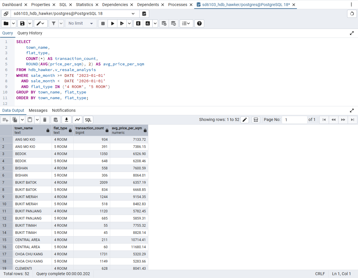
Central Area has the highest price per square metre for both 4-room and 5-room flats.
SELECT
    town_name,
    flat_type,
    COUNT(*) AS transaction_count,
    ROUND(AVG(price_per_sqm), 2) AS avg_price_per_sqm
FROM hdb_hawker.v_resale_analysis
WHERE sale_month >= DATE '2023-01-01'
  AND sale_month <  DATE '2026-01-01'
  AND flat_type IN ('4 ROOM', '5 ROOM')
GROUP BY town_name, flat_type
ORDER BY town_name, flat_type;
Mean of ratios: each sale's own price ÷ area is averaged. This is not total price over total area.
Half-open range: >= 2023-01-01 and < 2026-01-01 covers
exactly 36 months.
Result: SGD 10,714.41 over 211 four-room sales and SGD 11,680.14 over 60 five-room sales. The five-room sample is small, so the 9% gap is descriptive.
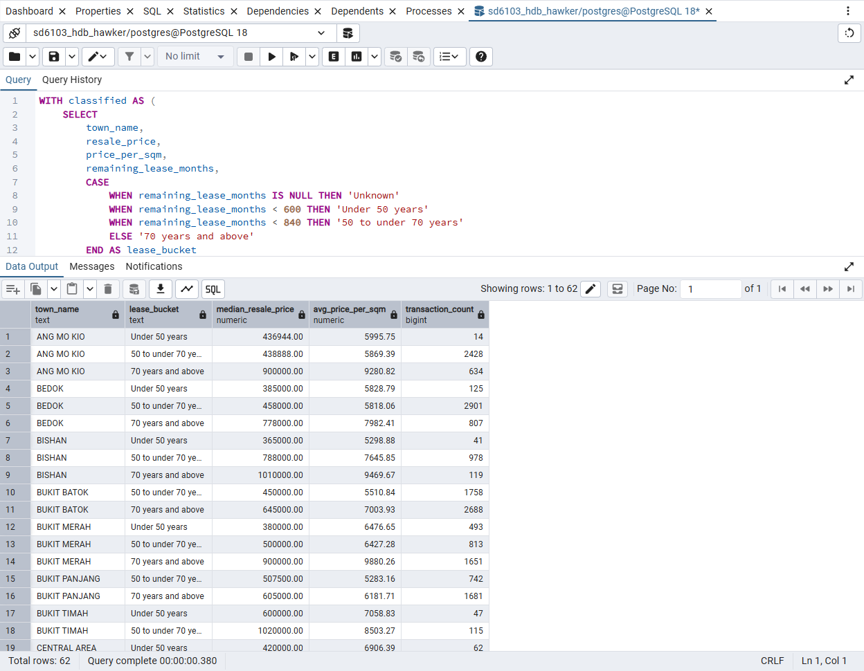
A longer remaining lease goes with higher prices, though the query does not hold flat type or location constant.
WITH classified AS (
    SELECT
        town_name,
        resale_price,
        price_per_sqm,
        remaining_lease_months,
        CASE
            WHEN remaining_lease_months IS NULL THEN 'Unknown'
            WHEN remaining_lease_months < 600 THEN 'Under 50 years'
            WHEN remaining_lease_months < 840 THEN '50 to under 70 years'
            ELSE '70 years and above'
        END AS lease_bucket
    FROM hdb_hawker.v_resale_analysis
    WHERE sale_month >= DATE '2023-01-01'
      AND sale_month <  DATE '2026-01-01'
)
SELECT
    town_name,
    lease_bucket,
    ROUND(
        (PERCENTILE_CONT(0.5) WITHIN GROUP (
            ORDER BY resale_price
        ))::numeric,
        2
    ) AS median_resale_price,
    ROUND(AVG(price_per_sqm), 2) AS avg_price_per_sqm,
    COUNT(*) AS transaction_count
FROM classified
GROUP BY town_name, lease_bucket
-- Buckets cover disjoint lease ranges, so the shortest lease orders
-- them; Unknown has no lease and sorts last.
ORDER BY town_name, MIN(remaining_lease_months) NULLS LAST;
Buckets: under 600 months, 600 to under 840, 840 and above, with Unknown kept apart. The CASE is written once, in the CTE.
Ang Mo Kio: median SGD 900,000 over 634 sales at 70 years and above, against SGD 438,888 over 2,428 sales at 50 to under 70.
Tampines has the largest 3-room flats, 71.24 m² on average.
-- Q3: Top 10 towns by average floor area of 3 ROOM sale observations.
-- Then return each selected town's highest 3 ROOM resale price per year.
-- The mean is transaction-weighted: each sale counts once, not each distinct flat profile.
-- Only sales in the 2023-2025 study window are used.

WITH three_room_sales AS (
    SELECT
        town_name,
        sale_year,
        floor_area_sqm,
        resale_price
    FROM hdb_hawker.v_resale_analysis
    WHERE flat_type = '3 ROOM'
      AND sale_month >= DATE '2023-01-01'
      AND sale_month <  DATE '2026-01-01'
),
top_towns AS (
    SELECT
        town_name,
        AVG(floor_area_sqm) AS avg_area_sqm
    FROM three_room_sales
    GROUP BY town_name
    ORDER BY avg_area_sqm DESC, town_name
    LIMIT 10
)
SELECT
    t.town_name,
    ROUND(
        CAST(t.avg_area_sqm AS numeric), 2
    ) AS avg_3room_area_sqm,
    s.sale_year,
    COUNT(*) AS yearly_transactions,
    MAX(s.resale_price) AS max_resale_price
FROM top_towns AS t
JOIN three_room_sales AS s
    ON s.town_name = t.town_name
GROUP BY
    t.town_name,
    t.avg_area_sqm,
    s.sale_year
ORDER BY
    t.avg_area_sqm DESC,
    t.town_name,
    s.sale_year;
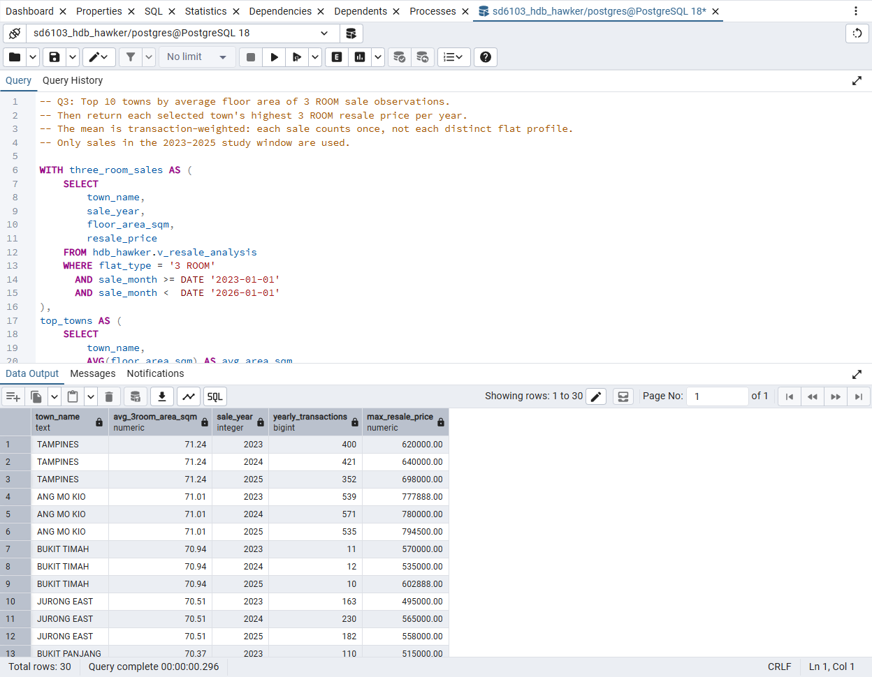
Reuse: the CTE three_room_sales feeds both the ranking and the yearly
maximum.
Tampines: its top 3-room price rises from SGD 620,000 (2023) to 698,000 (2025), about 12.58%. A maximum is one sale, not the typical price.
Near-centre sales are usually cheaper, but the gap reflects estate age more than proximity.
-- Q4: Nearest-overall hawker class, scoped to 2023-2025.
-- Keep NULL when a near/far comparison group is absent.
WITH price_summary AS (
    SELECT town_name, flat_type,
           AVG(resale_price) FILTER (
               WHERE hawker_proximity_class = 'near'
           ) AS near_avg,
           AVG(resale_price) FILTER (
               WHERE hawker_proximity_class = 'far'
           ) AS far_avg
    FROM hdb_hawker.v_resale_analysis
    WHERE sale_month >= DATE '2023-01-01'
      AND sale_month <  DATE '2026-01-01'
    GROUP BY town_name, flat_type
)
SELECT town_name AS town, flat_type,
       ROUND(near_avg, 2) AS avg_price_near_hawker,
       ROUND(far_avg, 2) AS avg_price_far_hawker,
       ROUND(100.0 * (near_avg - far_avg)
             / NULLIF(far_avg, 0), 2) AS price_diff_percentage
FROM price_summary
ORDER BY town_name, flat_type;
FILTER gives both averages in one pass. A town and flat type with no near or no far sales keeps NULL: 77 of the 130 rows. pgAdmin result
Why not a proximity discount: 60% of study sales are far, concentrated in newer estates the 2016 list misses. Near sales average 63.1 years of remaining lease, far sales 78.9 years.
Three of 26 towns exceed the budget, with no consistent pattern.
-- Q5: Average resale price per fresh-market proximity class, for the
-- towns whose overall average price (2023-2025 sales) is above the
-- SGD 750,000 budget. Every class of a qualifying town is shown.

WITH study_sales AS (
    SELECT
        town_name,
        fresh_market_proximity_class,
        nearest_fresh_market_distance_m,
        resale_price
    FROM hdb_hawker.v_resale_analysis
    WHERE fresh_market_proximity_class IS NOT NULL
      AND sale_month >= DATE '2023-01-01'
      AND sale_month <  DATE '2026-01-01'
),
towns_over_budget AS (
    SELECT
        town_name,
        AVG(resale_price) AS town_avg_price
    FROM study_sales
    GROUP BY town_name
    HAVING AVG(resale_price) > 750000
)
SELECT
    s.town_name,
    s.fresh_market_proximity_class AS proximity_class,
    COUNT(*) AS transactions,
    ROUND(AVG(s.resale_price), 2) AS avg_resale_price,
    ROUND(t.town_avg_price, 2) AS town_avg_resale_price,
    750000 AS budget_sgd
FROM study_sales AS s
JOIN towns_over_budget AS t
    ON t.town_name = s.town_name
GROUP BY s.town_name, s.fresh_market_proximity_class, t.town_avg_price
-- The classes cover separate distance ranges, so the closest sale in
-- each group puts them in near, medium, far order.
ORDER BY s.town_name, MIN(s.nearest_fresh_market_distance_m);
| Town over SGD 750,000 | Near | Medium | Far |
|---|---|---|---|
| Bishan town average 823,020 |
637,256 141 sales | 852,472 851 |
830,760 146 |
| Bukit Timah 897,986 |
897,986 162 | none | none |
| Central Area 760,729 |
805,810 450 | 549,414 96 |
none |
Whole towns: the budget is tested on the town average with HAVING, so a qualifying town shows every class it has and the classes can be compared.
Every sale has a class: it comes from the nearest centre with produce stalls at any distance. Limiting Q5 to near flats would leave one class and nothing to compare.
Reading: near is cheaper in Bishan and dearer in Central Area, so there is no general fresh-market premium or discount. pgAdmin result
Q6 joins all six tables: six towns have no listed centre within 500 m.
WITH active_blocks AS (
    -- Distinct blocks with at least one sale in the study window.
    SELECT DISTINCT
        t.town_id,
        t.town_name,
        b.block_id,
        b.latitude,
        b.longitude
    FROM hdb_hawker.town AS t
    JOIN hdb_hawker.hdb_block AS b
        ON t.town_id = b.town_id
    JOIN hdb_hawker.hdb_flat AS f
        ON b.block_id = f.block_id
    JOIN hdb_hawker.resale_transaction AS r
        ON f.flat_id = r.flat_id
    WHERE r.sale_month >= DATE '2023-01-01'
      AND r.sale_month <  DATE '2026-01-01'
),
block_coverage AS (
    -- LEFT JOIN retains blocks with no nearby matched centres.
    SELECT
        a.town_id,
        a.town_name,
        a.block_id,
        (
            a.latitude IS NOT NULL
            AND a.longitude IS NOT NULL
        ) AS has_coordinates,
        COUNT(h.hawker_id) AS nearby_hawker_count,
        COUNT(h.hawker_id) FILTER (
            WHERE h.market_produce_stalls > 0
        ) AS nearby_fresh_market_count
    FROM active_blocks AS a
    LEFT JOIN hdb_hawker.block_hawker_distance AS d
        ON a.block_id = d.block_id
       AND d.distance_m <= 500
    LEFT JOIN hdb_hawker.hawker_center AS h
        ON d.hawker_id = h.hawker_id
    GROUP BY
        a.town_id,
        a.town_name,
        a.block_id,
        a.latitude,
        a.longitude
)
SELECT
    town_name,
    COUNT(*) AS active_block_count,
    COUNT(*) FILTER (
        WHERE has_coordinates
    ) AS geocoded_block_count,
    COUNT(*) FILTER (
        WHERE NOT has_coordinates
    ) AS unknown_location_blocks,
    ROUND(
        AVG(nearby_hawker_count) FILTER (
            WHERE has_coordinates
        ),
        2
    ) AS avg_hawkers_within_500m,
    ROUND(
        AVG(nearby_fresh_market_count) FILTER (
            WHERE has_coordinates
        ),
        2
    ) AS avg_fresh_markets_within_500m,
    ROUND(
        100.0 * COUNT(*) FILTER (
            WHERE has_coordinates
              AND nearby_hawker_count = 0
        )
        / NULLIF(
            COUNT(*) FILTER (WHERE has_coordinates),
            0
        ),
        2
    ) AS pct_blocks_without_hawker_500m
FROM block_coverage
GROUP BY town_id, town_name
ORDER BY pct_blocks_without_hawker_500m DESC NULLS LAST,
         town_name;
In five of the six towns the coordinate file holds a newer centre outside the 2016 list. pgAdmin result
As sales grow fourfold, Q1 to Q3 slow modestly while Q4 and Q5 stay flat at about 1.8 seconds.
Reading the panels: each dot is one timed run, the line joins the mean of five. Every panel starts at zero and has its own scale; Q4 and Q5 take about ten times as long as the rest.
150 timings: 6 queries × 5 runs × 5 sizes, after one untimed warm-up per query. Client time covers execution and fetching every row.
Stage 1 ran first and is slower than stage 2 for Q1 to Q4 although it holds the least data, so we read the trend from stages 2 to 5: medians rise 138 to 177 ms (Q1), 234 to 277 (Q2) and 80 to 125 (Q3) while sales grow 3.53 times.
Runtime grows only where a plan scans a table that grows: the sales table grows 3.8 times, the distance table 0.9%.
Older files add sales but few new blocks, and the centre list is fixed, so the block-by-centre matrix barely moves: 1,015,248 to 1,024,608 rows.
| Query | Where the time goes, from EXPLAIN (ANALYZE, BUFFERS) | Effect of size |
|---|---|---|
| Q1 to Q3 | A sequential scan reads all 989,263 sales to keep the 78,670 in the window (7.95%). It is about a third of Q1's execution; joins, sorting and aggregation work on the same 78,670 rows at every size. | The scan grows with the table, from 3,296 to 12,512 pages. The rest does not. |
| Q4, Q5 | The nearest-centre views: DISTINCT ON reads 1,024,608 distance rows (798,012 for Q5), sorts each block's rows by distance and keeps the first. About 94% of the time before the final aggregation. | Flat. The input is the distance table, not the sales table. |
| Q6 | One sales scan to find the 9,385 active blocks, then the 3,634 distance rows within 500 m. | No trend: medians between 300 and 327 ms, within the run-to-run variation. |
This diagnosis named the two Task 4 candidates before any index was built:
one on sale_month, and one on block_hawker_distance in the order DISTINCT ON needs.
See the candidates.
Each candidate index targets one plan step that EXPLAIN showed to be expensive.
| Index | CREATE INDEX … ON | For | Plan step it targets | Why it should help |
|---|---|---|---|---|
| I1 | resale_transaction (sale_month) | Q1 to Q3 | Sequential scan of all sales to keep 7.95% | A B+ tree supports a range search. INCLUDE holds every column the queries read, allowing index-only evaluation. |
| I1b | resale_transaction (sale_month) | Q1 to Q3 | The same scan | Same search key, smaller entries, but each match needs a heap visit. Tests whether covering matters. |
| I2 | hdb_flat (flat_type, flat_id) | Q3 | Filter on 3 ROOM, 15.8% of profiles | A selective equality on a composite key. 4 ROOM and 5 ROOM together are 72%, too unselective for Q1. |
| I3 | block_hawker_distance | Q4, Q5 | Incremental Sort inside the nearest-centre views | The key is exactly the DISTINCT ON order, so rows arrive sorted. All three columns are in the key: index-only. |
| I4 | block_hawker_distance (distance_m) | Q6 | Scan of 1,024,608 pairs to keep 3,634 within 500 m | A highly selective range, 0.35% of rows. Few rows qualify, so an unclustered index wins; INCLUDE makes it index-only. |
Shaded rows are the two we kept. All five are B+ trees and unclustered. I2 and I3 are primary indexes, since their search key contains the table's primary key.
Priority: Q4 and Q5 are 41.4% and 38.6% of the six-query workload, so their plan step matters most.
Not tried: hash indexes, which cannot serve a range or an order; indexes on town (27 rows) or hawker_center (107 rows), which fit in one or two pages; CLUSTER, whose order PostgreSQL does not maintain.
Each of nine index configurations was timed 15 times per query, in three shuffled blocks that each hold a no-index control.
810 timings: 3 blocks × 9 configurations × 6 queries × 5 runs, on the largest database (989,263 sales, 337 MiB). The order shown is the order that ran. Each configuration is compared with the control of its own block, so a faster or slower hour affects both sides.
Same clock as Task 3: a new autocommit connection, no prepared statements, execution plus fetching every row. The Task 3 average is shown beside the control: 743 against 711 ms.
Two warm-up rounds, not one. In a pilot the first seconds of a new connection ran up to 2.5 times faster. With two rounds, run 1 is within 2% of runs 2 to 5.
VACUUM (ANALYZE) first. An index-only scan skips the heap only for pages marked all-visible. The control ran on the same vacuumed database.
Same answers. Every result was identical to Task 3 in every configuration.
Rule for reading a change: it counts as an index effect only if that query's plan changed. With an identical plan, differences reached 7.5% averaged over blocks, which we treat as run-to-run variation.
A copy, not the project database: the run used a TEMPLATE copy and dropped every Task 4 index at the end.
Only the two distance indexes speed up the workload; the sale_month indexes change plans but not the average.
Mean runtime in ms. Task 3 is the mean of 5 runs; every other column the mean of 15. Bold marks a query whose plan differs from the no-index plan. Other cells have the control's plan.
I3 alone takes 37% off the average and changes only the plans of Q4 and Q5. I1, I1b and I1+I2 change all six plans and end at −1%, −1% and −2%.
The Excel bar charts the specification asks for: Figure 9 (Q1, Q2, Q3, Q6) and Figure 10 (Q4, Q5).
I3 hands the nearest-centre view its rows already sorted, so the sort disappears and Q4 falls from 1,796 to 939 ms.
Q4 without a Task 4 index
- Read block_hawker_distance1,024,608 rows in primary-key order (block_id, hawker_id)
- Join to blocks and centreskeeps geocoded pairs
- Incremental Sorteach block's rows by distance_m, hawker_id: 355 ms of its own
- Uniquefirst row per block: 9,852 nearest centres
- Hash, then join to the salesrepeated in every parallel process
Q4 with I3
- Index Only Scan using ix_bhd_block_distance1,024,608 entries in (block_id, distance_m, hawker_id) order; 78 heap fetches
- Join to blocks and centresorder is preserved
- Uniquereads the sorted stream directly
- Hash, then join to the salesplan is still parallel
| Mean of 15 runs | No index | I3 | Faster |
|---|---|---|---|
| Q4 | 1,796 ms | 939 ms | 48% |
| Q5 | 1,623 ms | 904 ms | 44% |
| Six-query average | 711 ms | 446 ms | 37% |
Why index-only: all three columns are in the key and the visibility map is set after VACUUM, so the heap is hardly touched.
Why only half: the index changes the order in which rows arrive, not how many are read. All 1,024,608 pairs are still read to find 9,852 nearest centres, in each of three processes.
Going further needs a different view, for example a materialized nearest-centre table. We did not benchmark it, because Task 4 compares indexes on unchanged queries.
The sale_month index makes Q1's scan cheaper but the query 17% slower, because the planner drops the parallel plan.
Q1 without a Task 4 index
- Parallel Seq Scan on resale_transactiontests 989,263 rows, keeps 78,670
- Parallel Hash Join to flat profilesin three processes
- Sort by town and flat typein three processes
- Gather Mergecombines the three sorted streams
- Aggregate52 rows
Q1 with I1
- Index Only Scan using ix_resale_sale_month_covonly the 78,670 window rows; 0 heap fetches
- Hash Join to flat profileshash table on 106,498 profiles, one process
- Sort by town and flat type52,280 rows, one process
- Aggregate52 rows
Cause: with only 78,670 index entries to read, the cost model prefers a serial plan. It counts page reads, but every page is already in memory, so the I/O saved is small beside the lost parallel CPU work.
Q5 loses parallelism the same way, and its serial part includes the nearest-centre computation.
I1b, without INCLUDE, uses a Bitmap Heap Scan: 6.7 instead of 45.8 MiB, but Q1 is 26% slower.
We keep I3 and I4: the six-query average falls from 711 to 435 ms for 79 MiB of index.
I3 and I4 do not interact. They serve different plan steps and keep both gains: Q4 48%, Q5 43% and Q6 22% faster than the control. Every query is faster than in Task 3 (743 ms on average).
Why not all four, which was fastest at 414 ms:
The extra 52.9 MiB is two-thirds more index storage for about 5% less runtime.
I1 sits on the one table that grows with every monthly resale file, so it is the most expensive to maintain. The distance table changes only when blocks or centres are added.
Its benefit depends on the planner's choice between a parallel and a serial plan, which alone made Q1 17% and Q5 9% slower.
Break-even: with equal weights elsewhere, all four stops paying off once Q5 runs about 2.2 times as often as each other query. An index belongs to the whole workload.
Five limits bound what these results can claim.
| Limit | What follows from it |
|---|---|
| Distance is a straight line, not a walking route | Barriers and paths are ignored. The 500 m and 1,000 m bands are project definitions. |
| The centre list is the 2016 NEA master, 107 centres | Newer centres such as One Punggol and Fernvale are missing, so 60% of study sales are far and the far group is concentrated in newer estates. |
| Distances and stall counts are one snapshot | The same values are applied to every sale year from 1990 to 2026. |
| The queries are descriptive | None holds flat type, lease or location constant. Q4's gap mixes estate age with proximity; the results are associations, not effects. |
| Timings are warm-cache client timings on one Windows workstation | Differences of a few tens of milliseconds are within noise. The faster first seconds of a new connection were handled with extra warm-up, and their cause was not established. |
What holds despite them: all 989,263 source sales are retained in six BCNF tables, the runtime diagnosis from Task 3 predicted which index would help, and the index experiment confirmed it against a control in the same run.
Each line points to the slide that answers it.